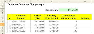
I used to deal with incoming shipment of imported parts. With current economic slow down, our warehouse storage was full, such lead to stranded container at Port. I have to monitor number of
day balance before detention charges imposed, in our case we have 30 days free period.
Normally we used to just minus current date to arrival date, most of the time we only see numbers.
Recently I came across excel function i.e "
Conditional formatting", from that day, it looks more colorful , more colors to show level of critical. Here how the function work.
Conditional formatting enables you to quickly and easily color coded your information based on parameter that you set. It saves time by emphasizing exactly what you want to see.
Select the cells to which you want to add conditional formatting. In our example, we selected cells F6 through F9.
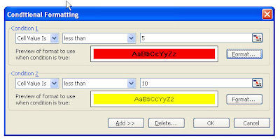
Add conditional formatting
- On the Format menu, click Conditional Formatting.
In the Condition area, do one of the following:
- To change the formatting based on a value, select Cell Value Is, select a condition from the drop-down menu, and then enter a number or a formula. If you enter a formula, start it with an equal sign (=).
- To change the formatting based on a formula that evaluates to TRUE or FALSE, select Formula Is, and then enter a formula.
In our example, we chose Cell Value Is, selected the condition less than, and entered 5.
- Click Format.
Select the formatting you want to apply when the cell value meets the condition that you specified, or when the formula value returns TRUE.
In our example, we changed the Cell color to red & the text to bold.
- Click OK.
To add another condition, click Add, and repeat steps 3 through 6.
In our example, we added a second condition stating that if the Cell Value Isless than 10, the cell will be colored to yellow.
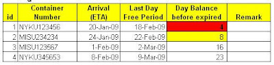
This is the result.
We can have up to three condition.
So, have a try and give your report some value.


 Date & time in two different cell
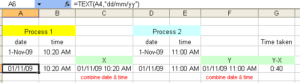 First
First

 if the date format not converted to text, date will be define as number
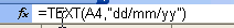 if the date format not converted to text, date will be define as number


