Friday, November 20, 2009

Combine text format date and time to date_time format

Recently my friend do ask me about combining date and time which written in two different column. The purpose was to find different between those 2 date/time i.e time taken to complete a process.

Sample of original data as follow;
Date & time in two different cell
Purpose : To find time difference between process 1 & 2


The solution;First
i. Convert date and time format to text, use TEXT function if the date format not converted to text, date will be define as number
such as 40,118 for 1st Nov 2009 instead of 1/11/09

Second
i. Combine both date & time text using CONCATENATE function,
tips : follow standard date & time format setting i.e dd/mm/yr_hh:mm am/pm

Wednesday, March 11, 2009

Text date convert to date format


Previously I had post one method of doing this, show me.


Today I would like to share other way to perform this action
1. Select cell range (data range where we want to convert)

2. Go to Menu - Data, select "Text to column", the working box as follow;

3. Select "Delimited", press Next
4. Result

The next now splitted to 3 column which consists of day, month & year value in each cell.
example 11.05.2009 will be splitted to 11, 5 and 2009

5. Use excel "Date" function, date(year,month,day)
Set day to 11, month to 5 and year 2009

6. The result was a date format which could be change to follow date format
i.e (format.. cells...date.. select format that we required)

Sunday, February 22, 2009

What You Can Do With Excel?

With the numerous features available in Excel, you can use it widely. Some of them are:

  • Creating invoice, purchase order, DO, etc
  • Presenting data in different types of chart formats!
  • Get the latest prices for stocks, percentage change in stock value, etc.
  • Calculate a loan due date or how many days you have been alive?
  • Calculate future value of your saving or amount to keep in order to get targeted amount by end of saving... through excel functions.
  • And many more....

Those tasks can have a 'build-in calculator' that will automatically calculate the figure based on the pre-set formula with 100% accuracy. This is the biggest advantage of computer spreadsheet compare with manual when dealing with figures.

Thanks to the powerful Excel feature – Formulas and Functions! …and you can learn it in the online Excel tutorials help below.

If you have used the correct functions and formulas within the spreadsheet, the computer automatically re-calculate the end values.

Friday, February 13, 2009

Adding Visual Control To Your Report through "traffic light"

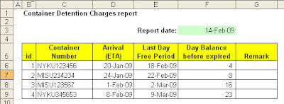
I used to deal with incoming shipment of imported parts. With current economic slow down, our warehouse storage was full, such lead to stranded container at Port. I have to monitor number of day balance before detention charges imposed, in our case we have 30 days free period.

Normally we used to just minus current date to arrival date, most of the time we only see numbers.
Recently I came across excel function i.e "Conditional formatting", from that day, it looks more colorful , more colors to show level of critical. Here how the function work.

Conditional formatting enables you to quickly and easily color coded your information based on parameter that you set. It saves time by emphasizing exactly what you want to see.

Select the cells to which you want to add conditional formatting. In our example, we selected cells F6 through F9.

Add conditional formatting

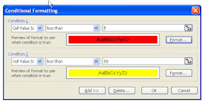
  1. On the Format menu, click Conditional Formatting.
  2. In the Condition area, do one of the following:

    • To change the formatting based on a value, select Cell Value Is, select a condition from the drop-down menu, and then enter a number or a formula. If you enter a formula, start it with an equal sign (=).
    • To change the formatting based on a formula that evaluates to TRUE or FALSE, select Formula Is, and then enter a formula.

    In our example, we chose Cell Value Is, selected the condition less than, and entered 5.

  3. Click Format.
  4. Select the formatting you want to apply when the cell value meets the condition that you specified, or when the formula value returns TRUE.

    In our example, we changed the Cell color to red & the text to bold.

  5. Click OK.
  6. To add another condition, click Add, and repeat steps 3 through 6.

  7. In our example, we added a second condition stating that if the Cell Value Isless than 10, the cell will be colored to yellow.


This is the result.

We can have up to three condition.

So, have a try and give your report some value.

Tuesday, February 3, 2009

Remove Blank Rows

This will show you how to remove blank row, this normally happen when you downloaded data (such as from SAP system) to Ms Excel
First
Highlight your range and go to Edit>Go to>Special and select "Blanks"
Then
"Ok" now go to Edit>Delete or Ctrl+Shift+= (equal)
and then select "Entire row" from the "Delete" dialog
and click "Ok".

Adding Hidden Text to Formulas

Imagine you have a formula like: =$2018+$1056-4*$120.

When you initially wrote it you knew what each number represented, but you come back later and can't remember.

Add a hidden note to your formula by using the N() formula

i.e. =$2018+$1056-4*$120+N("My Wage+Bonus-4 weekly loan repayments").

The N() function will convert text to zero.

But be aware not to put * instead of + infront of N i.e *N(" ") since this will be return the amount as zero (similar like numbers multiple with zero value).

Sunday, January 18, 2009

Shortcut with CTRL & SHIFT Key

Let share about shortcuts

Practicing the CTRL SHIFT shortcuts will save tons of time:


CTRL SHIFT :
Enters the time
CTRL SHIFT &
Creates an outline box around whatever you select
CTRL SHIFT _
Removes the outline box around whatever has an outline
CTRL SHIFT *
Highlights all the text surrounding the cell filled with data or numbers
CTRL SHIFT !
Applies the number format to selected cells
CTRL SHIFT %
Applies the percentage format to the selected cells
CTRL SHIFT #
Applies the date format to the selected cells
CTRL SHIFT @
Applies the time format to the selected cells
CTRL SHIFT (
Unhide columns that are selected
CTRL SHIFT )
Unhide rows that are selected


Here are a few other CTRL shortcuts that can save time:

CTRL ;
Enters the date
CTRL 9
Hide Rows selected
CTRL 0
Hide Columns selected
CTRL D
Fills down current formula into all adjacent cells; this avoids copying first
CTRL K
Insert a hyperlink

Tuesday, January 13, 2009

Continue_Create List of Day


Here come the picture of previous tips for batter understanding.

Saturday, January 10, 2009

How to build List of Day (Sun, Mon, Tue) continuously

Happy New Year 2009... there will be lots more post the year.

Recently I am doing my macro project on Yearly Attendance Leave Chart (in Ms Excel). One of the logic is to assign day for each date and to identify Saturday and Sunday, so that it will be highlighted as different color in the chart. The issue now is how to identify Sunday & Saturday the fastest way instead of assign it manually. Here is the way;
1. Build list of date
i. Key in 1st date ex 01/01/09 (DD/MM/YR) - cell(A2)
ii. Key in 2nd date ex 02/01/09 (DD/MM/YR) - cell(A3)
iii. Select both cells, place the cursor at the right corner of the selection till the cursor mark as
"+" and drag cell downwards.
2. Build list of day
i. Key in 1st day ex Thursday - cell(B2)
ii. Key in 2nd day ex Friday - cell(B3)
iii. Select both cells, place the cursor at the right corner of the selection till the cursor mark as
"+" and drag cell downwards.
tips: Fastest way, once (+) appear, double click the (+) sign, the list will be copied to the
following cell following the trend of selected cells.

Next posting : Video how to perform this post.